Hi,
We've just released 6.9 which fully supports conditional formats
in xlsx files. You can use APIMate to know how to add formats with the API, and they will be preserved and exported to pdf.
Thank you for your work. I tried it and it works!
But now I have another question concerning conditional formats. Is it possible to update the cell reference while the conditional format is being copied? I use 3 columns to show some data (columns A,B,C). Now i want to use a conditional format for column A which depends on the according data in column C. So I created a conditional format at column A that looks like "value <> C1". But unfortunately the reference to the cells in column C is not updated. So I have 100 data rows with 100 conditional formats which are all referencing C1. But what I would like to have are data rows with conditional formats that referencing their according cell in column C (so C1 to C99).
Best regards
Hi,
All references should be updated, same as in Excel.
Are you sure you are setting "value <> C1" and not "value <> $C$1" ? If you are setting the second, indeed the reference won't move when you copy it, because that is the meaning of "$". But if you don't use "$", it should move.
Another thing, just in case, is that you should enter the formula without quotes: "values <> c1" is a string and it won't move.
Here is a simple example code which sets a value and copies it down. As you can see in the generated file, the references move too:
program Project15;

{$APPTYPE CONSOLE}

{$R *.res}

uses
  System.SysUtils,
  VCL.FlexCel.Core,
  FlexCel.XlsAdapter;

var
  xls: TXlsFile;
  Ranges: TArray<TXlsCellRange>;
  Rules: TArray<IConditionalFormatRule>;
  ExpressionRule: IConditionalExpressionRule;
  CFDef: TConditionalFormatDefStandard;
begin
  xls := TXlsFile.Create(true);
  try
    xls.NewFile(1, TExcelFileFormat.v2016);
    //Set the cell values
    xls.SetCellValue(1, 1, TFormula.Create('=RANDBETWEEN(1, 2)'));
    xls.SetCellValue(1, 3, 1);

    //Conditional Formats
    Ranges := TArray<TXlsCellRange>.Create(
      TXlsCellRange.Create(1, 1, 1, 1)
    );

    Rules := nil;  //SetLength will resize the array in place. We set it to nil first to create a new array.
    SetLength(Rules, 1);
    ExpressionRule := TConditionalExpressionRule_Create(1, false, '=A1=C1');
    CFDef := ExpressionRule.FormatDef;
    CFDef.ApplyFill.BgColor := true;
    CFDef.Fill.BgColor := TExcelColor.FromTheme(TThemeColor.Accent6, 0.399945066682943);
    Rules[0] := ExpressionRule;

    xls.AddConditionalFormat(TConditionalFormat.Create(Ranges, Rules, false));

    xls.InsertAndCopyRange(TXlsCellRange.Create(1, 1, 1, 1), 2, 1, 10, TFlxInsertMode.ShiftRowDown);
    xls.Save('..\..\result.xlsx');
  finally
    xls.Free;
  end;

end.
Hi,
my post wasn't really clear. I created a conditional format via Excel, I am not creating it programmatically.
In the following picture you see my settings for the conditional format for cell A1 (it is in German but I think you can still read the settings). As you can see, i wrote C1 ("Zellwert" = "cell value" and "ungleich"="not equal" ) :
And after report creation every data cell (A1 to A99) referencing C1. I am using Excel 2016.
Sorry, I can't see the images. Can you repost them?
Ok, I got the images by email, thanks.
Creating the conditional formats with Excel or FlexCel shouldn't change anything: In fact to create the code I sent above I originally did it with a file I created in Excel, then converted with APIMate to code so I wouldn't have to attach a file.
But it should work the same with a file created in Excel. You can get a simple example of a file created with the settings in your screenshot here:
http://www.tmssoftware.biz/flexcel/samples/cf_propagation.zip
And you will see that only values that are different from the same value in column C are highlighted.
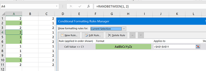
Maybe the confusion comes from the fact that Excel always displays the formula as "<>C1"?:
If that is the issue, it is just that when using relative references (without $) Excel shows the top-left cell, but it applies to the cell where it is at. So the relative reference "C1" applied in A4,means "C4". There is no really other way to show it, Excel wouldn't be able to show =C1, =C2, =C3... in that dialo when you show the rule. but if the reference is relative, it will be applied relative to the cell.
Here there is a little difference between Excel and FlexCel: We always consider the top at A1, so to enter a cell that is 2 columns to the left and in the same row you would enter C1. In Excel it uses the top-left cell of the range, which in this case is also A1, but if it was say B5, then for 2 columns to the left you would enter D5. This is all in how you enter the formulas, we believe that a fixed origin at A1 is the easiest. But the result of course is the same, only that you would enter the formula "=C1" in FlexCel, and it would show as =D5 in Excel if the top left is B5.
It was indeed a display problem. In every row the condition was true, so the format has always been applied and the Excel dialog always showed the reference to C1. That are the reasons I thought the conditional formats references were not updated. But everything is working. Sorry for causing this effort und thank you again!
